SQL Patterns That Actually Show Up in Interviews (All 10, With Code)

Nobody fails a SQL interview because they don’t know the syntax. They fail because they stare at a question about “users with a 5-day login streak” and...

Nobody fails a SQL interview because they don’t know the syntax. They fail because they stare at a question about “users with a 5-day login streak” and don’t recognize it as the exact same problem as “continuous subscription periods” and “consecutive winning games” — three phrasings of one pattern with one trick. The engineers who breeze through SQL rounds aren’t faster typists or syntax savants. They’ve seen the patterns enough times that a novel-sounding question instantly collapses into “oh, that’s gaps-and-islands” — and then the SQL is the easy part.

There are about ten of these patterns, and they cover the overwhelming majority of what product companies actually ask. This is a tour of all ten — the keyword that gives each one away, the core trick, real SQL, and the follow-up the interviewer asks when you get the first version right. The goal isn’t to memorize ten queries; it’s to build the recognition reflex so that in the room, you spend your time on the interesting variation instead of rediscovering the base pattern from scratch. If you want the deeper argument for why this recognition skill matters more than raw syntax, I’ve made it in why senior engineers write SQL differently.

One thing worth pinning to the wall before we start — the logical execution order of a query, because half of “why doesn’t my WHERE see my alias” questions dissolve once you know it: FROM → JOIN → WHERE → GROUP BY → aggregates → HAVING → SELECT → ORDER BY.

The whole game in one table: interviewers rarely name the pattern, but the words they use give it away. Train yourself to hear the keyword and reach for the trick.

1. Gaps and islands (consecutive sequences)

Keywords: consecutive, streak, continuous, sessions, “5 days in a row.” This is the one that trips people up most, and the trick is almost magical once it clicks: subtract a row number from the ordered date. Consecutive dates produce the same constant; a gap shifts it, creating a new group.

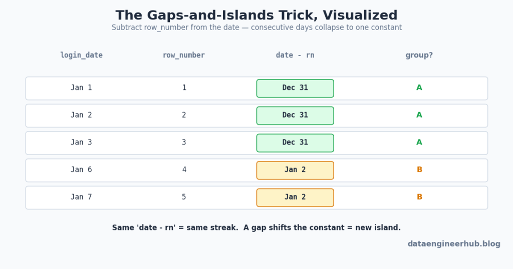
Why it works: for consecutive days the row number grows in lockstep with the date, so date − rn is constant. The moment a day is skipped, the constant jumps — and that jump is your new streak boundary.

WITH distinct_logins AS (
  SELECT DISTINCT user_id, login_date FROM logins
),
numbered AS (
  SELECT user_id, login_date,
         ROW_NUMBER() OVER (PARTITION BY user_id ORDER BY login_date) AS rn
  FROM distinct_logins
),
login_groups AS (
  SELECT user_id, login_date,
         DATE_SUB(login_date, INTERVAL rn DAY) AS grp
  FROM numbered
)
SELECT user_id,
       MIN(login_date) AS streak_start,
       MAX(login_date) AS streak_end,
       COUNT(*)        AS streak_length
FROM login_groups
GROUP BY user_id, grp
HAVING COUNT(*) >= 5
ORDER BY user_id;

The follow-up: “what if you need to detect the gaps themselves, not the streaks?” Switch to LAG() — compare each row to the previous login, flag where the difference isn’t 1 day, and cumulative-sum those flags into group IDs. Same idea, different vehicle. Note the DISTINCT up front: duplicate logins on the same day would silently break the row-number arithmetic.

2. Top-N per group

Keywords: top 3 per department, highest/lowest per group, latest record, first/last. The single most common window-function question. Partition by the group, order by the metric, filter on the rank.

WITH ranked AS (
  SELECT *,
         ROW_NUMBER() OVER (PARTITION BY department ORDER BY salary DESC) AS rn
  FROM employees
)
SELECT * FROM ranked WHERE rn <= 3;

The follow-up you must nail: “what if two people tie on salary?” That’s the interviewer probing whether you know the three ranking functions — and this is one of the most common trip-ups, so know it cold: ROW_NUMBER() gives 1,2,3 with an arbitrary tiebreaker; RANK() gives 1,1,3 (ties share a rank, next rank skips); DENSE_RANK() gives 1,1,2 (ties share, no gap). If the question is “top 3 salaries” and ties should all count, you want DENSE_RANK(), not ROW_NUMBER(). For the “latest record per user” variant, it’s the identical shape with ORDER BY created_at DESC and WHERE rn = 1.

3. Running totals / cumulative metrics

Keywords: running total, cumulative, so far, progressive. The frame does the work: SUM(x) OVER (ORDER BY dt ROWS BETWEEN UNBOUNDED PRECEDING AND CURRENT ROW).

WITH daily_revenue AS (
  SELECT DATE(created_at) AS order_date, SUM(amount) AS revenue
  FROM orders
  GROUP BY DATE(created_at)
)
SELECT order_date,
       SUM(revenue) OVER (
         ORDER BY order_date
         ROWS BETWEEN UNBOUNDED PRECEDING AND CURRENT ROW
       ) AS running_total
FROM daily_revenue;

The follow-up: “now show each user’s running total and the global running total in the same query.” That tests whether you understand that two window functions can carry different PARTITION BY clauses side by side — a per-user frame partitioned by user_id, and a global frame with no partition — which usually means aggregating to user-day and day grains first, then combining.

4. Event → state transformation

Keywords: headcount over time, active subscriptions per day, “build the metric then track it.” Here the metric doesn’t exist in the data — you construct it from events. The classic is daily headcount: turn each hire into +1 and each termination into −1, then take a running sum over a date spine.

WITH RECURSIVE date_spine AS (
    SELECT MIN(hire_date) AS dt FROM employee
    UNION ALL
    SELECT DATE_ADD(dt, INTERVAL 1 DAY) FROM date_spine
    WHERE dt < CURRENT_DATE()
),
changes AS (
    SELECT hire_date AS dt, +1 AS delta FROM employee
    UNION ALL
    SELECT termination_date AS dt, -1 AS delta
    FROM employee WHERE termination_date IS NOT NULL
),
daily_change AS (
    SELECT dt, SUM(delta) AS tdelta FROM changes GROUP BY dt
)
SELECT d.dt,
       SUM(COALESCE(c.tdelta, 0)) OVER (
         ORDER BY d.dt ROWS BETWEEN UNBOUNDED PRECEDING AND CURRENT ROW
       ) AS headcount
FROM date_spine d
LEFT JOIN daily_change c ON d.dt = c.dt
ORDER BY d.dt;

The “+1/−1 delta then running sum” trick generalizes to any state-from-events problem: concurrent sessions, active subscriptions, inventory on hand.

5. Rolling / moving windows

Keywords: 7-day moving average, 30-day active users, trailing metric. Same window machinery as running totals, but a bounded frame. The gotcha that separates candidates: ROWS BETWEEN 6 PRECEDING AND CURRENT ROW is 7 rows, not 6.

SELECT sale_date, daily_sales,
       AVG(daily_sales) OVER (
         ORDER BY sale_date
         ROWS BETWEEN 6 PRECEDING AND CURRENT ROW
       ) AS moving_avg_7d
FROM daily_sales;

Window frames are worth truly internalizing, because half these patterns are just different frame boundaries over the same OVER() skeleton:

Every rolling metric is just a choice of frame boundaries relative to the current row. And the ROWS-vs-RANGE distinction at the bottom is a favorite senior-level probe — worth knowing why one is deterministic.

The ROWS-vs-RANGE trap: the default frame for SUM() OVER (ORDER BY dt) is actually RANGE, which groups all rows sharing the same ORDER BY value into one step — so two orders on the same date both get the day-end total, not their individual accumulation. ROWS treats each physical row independently. For running totals and time series, prefer ROWS to avoid unintended grouping on ties; being able to explain that difference unprompted signals real depth.

6. Cohort / retention analysis

Keywords: retention, cohort, week 0 / week 1, signup behavior. Ubiquitous at product companies. The shape is always: assign each user a cohort (their first-activity period), then measure activity by offset from that cohort.

WITH user_cohort AS (
  SELECT user_id, DATE_TRUNC('week', MIN(activity_date)) AS cohort_week
  FROM user_activity GROUP BY user_id
),
user_activities AS (
  SELECT a.user_id, c.cohort_week,
         DATE_TRUNC('week', a.activity_date) AS activity_week
  FROM user_activity a
  JOIN user_cohort c ON a.user_id = c.user_id
),
cohort_size AS (
  SELECT cohort_week, COUNT(DISTINCT user_id) AS total_users
  FROM user_cohort GROUP BY cohort_week
)
SELECT ua.cohort_week,
       DATEDIFF('week', ua.cohort_week, ua.activity_week) AS weeks_since_signup,
       COUNT(DISTINCT ua.user_id) AS active_users,
       COUNT(DISTINCT ua.user_id) * 1.0 / cs.total_users AS retention_rate
FROM user_activities ua
JOIN cohort_size cs ON ua.cohort_week = cs.cohort_week
GROUP BY ua.cohort_week, weeks_since_signup, cs.total_users
ORDER BY ua.cohort_week, weeks_since_signup;

The three-CTE structure — cohort assignment, activity-with-offset, cohort size for the denominator — is the reusable skeleton. Retention rate is just active-at-offset divided by the week-0 size.

7. Self-join logic

Keywords: compared to previous, more than their manager, bought A but not B. Any time you compare rows within the same table. The “A but not B” version is a clean anti-join:

SELECT DISTINCT a.user_id
FROM purchases a
LEFT JOIN purchases b
  ON a.user_id = b.user_id AND b.product = 'B'
WHERE a.product = 'A' AND b.user_id IS NULL;

The trap here is NULLs. The instinct is often WHERE user_id NOT IN (SELECT user_id FROM purchases WHERE product='B') — but if that subquery returns even one NULL, NOT IN yields zero rows, silently. The LEFT JOIN ... IS NULL anti-join above is immune. Many “compare to previous row” self-joins are also better expressed with LAG(), which is cheaper than a correlated subquery and reads more clearly.

8. Time-series expansion (date spine)

Keywords: daily trend, fill missing dates, continuous timeline, “even days with zero.” The fix for gaps in a report is to generate the complete calendar and LEFT JOIN your data onto it, so missing periods become explicit zeros instead of vanishing rows.

WITH RECURSIVE months AS (
    SELECT DATE_FORMAT(MIN(hire_date), '%Y-%m-01') AS month_start FROM employees
    UNION ALL
    SELECT DATE_ADD(month_start, INTERVAL 1 MONTH) FROM months
    WHERE month_start < DATE_FORMAT(CURRENT_DATE(), '%Y-%m-01')
)
SELECT m.month_start, COALESCE(SUM(x.metric), 0) AS metric
FROM months m
LEFT JOIN some_table x ON DATE_FORMAT(x.dt, '%Y-%m-01') = m.month_start
GROUP BY m.month_start
ORDER BY m.month_start;

The production aside worth saying out loud: recursive date spines that recompute headcount by rescanning all employees every month are fine in an interview but expensive at scale. Mentioning that you’d back this with a precomputed monthly_headcount snapshot table in production — built by an incremental pipeline rather than recomputed each run — is exactly the kind of comment that separates a senior candidate, and it ties directly to not reprocessing what didn’t change.

9. Percentiles / distribution

Keywords: top 10%, percentile, ranking distribution. This is where NTILE(), PERCENT_RANK(), and DENSE_RANK() live. “Top 10% of employees by rating” has a naive form and a fair form, and the interviewer usually wants the fair one:

-- Fair version: handles ties at the cutoff correctly
WITH latest_rating AS (
  SELECT emp_id, rating,
         ROW_NUMBER() OVER (PARTITION BY emp_id ORDER BY review_date DESC) AS rnk
  FROM performance_reviews
),
ranked AS (
  SELECT *,
         DENSE_RANK() OVER (ORDER BY rating DESC) AS bucket,
         COUNT(*)     OVER () AS total_count
  FROM latest_rating WHERE rnk = 1
)
SELECT * FROM ranked WHERE bucket <= CEIL(0.10 * total_count);

NTILE(10) forces exactly ten equal-sized buckets (take bucket 1); the DENSE_RANK approach is fairer when many people share the boundary rating. The killer follow-up is point-in-time correctness: “employees change departments over time — attribute each rating to the department they were in then.” That forces a slowly-changing-dimension join on a date range (start_date <= review_date < end_date) instead of a naive join to the employee’s current department — and getting that right is a strong signal.

10. Detect overlapping date ranges

Keywords: booking conflicts, overlapping subscriptions, double-booked, schedule clash. The elegant move is to reason about when ranges don’t overlap, then invert. Two ranges miss each other only if one ends before the other starts:

-- Non-overlap:  a.end < b.start  OR  b.end < a.start
-- Invert (De Morgan) -> the standard overlap condition:
SELECT s1.customer_id,
       s1.subscription_id AS sub_1,
       s2.subscription_id AS sub_2
FROM subscriptions s1
JOIN subscriptions s2
  ON s1.customer_id = s2.customer_id
 AND s1.subscription_id < s2.subscription_id   -- avoid self- and duplicate pairs
 AND s1.end_date >= s2.start_date
 AND s2.end_date >= s1.start_date;

Two details interviewers check: the s1.id < s2.id condition (so you don’t compare a row to itself or count each pair twice), and that you derived the overlap condition rather than memorized it — walking through the two non-overlap cases and applying De Morgan’s law is the move that earns the nod.

Putting it together: the combined question

Real interviews often stack two or three patterns. “Monthly revenue for completed 2025 orders, with the change vs the previous month, showing all 12 months even when revenue is zero” is three patterns at once: conditional filtering, a date spine (all 12 months), and LAG() for the month-over-month delta — over a base that first aggregates order_items to order grain before summing to month grain. If you can see it as “aggregate → spine → LAG” instead of one intimidating blob, you’ve already won. The recognition reflex is the whole skill; the syntax is just spelling.

The gotchas nobody warns you about

NOT IN with a NULL returns nothing. One NULL in the subquery and NOT IN silently yields zero rows. Use NOT EXISTS or a LEFT JOIN ... IS NULL anti-join for exclusions, every time.

ROWS ≠ RANGE, and the default is RANGE. SUM() OVER (ORDER BY dt) groups tied values into one step. For a true row-by-row running total, spell out ROWS BETWEEN UNBOUNDED PRECEDING AND CURRENT ROW.

“6 PRECEDING” is a 7-row window. Off-by-one on frame bounds silently produces the wrong average. Count the current row.

ROW_NUMBER vs RANK vs DENSE_RANK is a tie question in disguise. When the interviewer says “what if they tie,” they’re testing which one you’d swap to. Have the 1,2,3 / 1,1,3 / 1,1,2 distinction ready.

Wrapping a date column in a function kills index/pruning use. Prefer hire_date >= DATE_SUB(CURRENT_DATE(), INTERVAL 6 MONTH) over TIMESTAMPDIFF(MONTH, hire_date, ...) <= 6 — same logic, but the range predicate can use metadata the function form throws away.

The one principle

You don’t pass a SQL interview by knowing more syntax — you pass it by recognizing that the strange-sounding question in front of you is one of about ten patterns you’ve already solved a dozen times. Learn the keyword that gives each pattern away, learn the one core trick behind it, and practice the recognition until it’s instant. Then the interview stops being a memory test and becomes what it should be: a conversation about the interesting variation, conducted in a language you already speak fluently.